
GIS Data Catalog
2021 LiDAR Digital Surface Model (DSM) Elevation and Hillshade
Learn how to get an ArcGIS Online account 🗺
Use this Data
|
Links
How to use in ArcGIS Pro |
|
| Sharing Status | Not Public |
Summary
Useful for defining top of vegetation location and its general height above ground surface, as well as defining elevations of manmade features such as buildings, structures and highway overpasses.
As no points are removed the high point density of the data strongly delineates edges of features, especially buildings.
Data are also useful for calculating separation distance between this data and either of the two other elevation surfaces in this suite - bare-earth elevation model and last-return elevation data.
This separation distance has potential applications in determining biomass with other potential uses in concert with supplemental data sets, particularly orthoimagery and classified imagery.
These data was processed through a series of quality control steps by both the vendors and clients; however, the data were not edited to define a true modelled surface, but rather represent a data point cloud.
Due to this some erroneously high points are occassionally found, usually bird-strikes, that have not been edited out during this edition of the data.
The number of these points is very limited.
Users need to be more aware that the data represent the first-return and may not necessarily represent the highest point of a feature.
This can have implications in difference calculations between surfaces, especially when done at any resolution greater than the point level.
As with the bare-earth data set, water areas are always suspect and elevation values from these surfaces should not be considered valid.
Users must make careful review of the fitness of these data for their particular use.
For many purposes a site- and use-specific field survey will be necessary.
Description
First-return LiDAR data elevation values consisting of the first return in a multiple-return LiDAR pulse or the sole return for a single-return pulse.
These data are directly extracted from the raw data and are not processed to remove vegetation.
Depicts the top of all surfaces whether bare-earth, non-elevated manmade surfaces, elevated vegetative, or elevated manmade surfaces.Also called top-of-vegetation surface or full-feature Though the data is referred to as a digital surface model (DSM), the data actually represent a 'point cloud' defining the top-of-surface and points do not necessarily represent the highest surface for a specific location.Data is stored as variably-spaced point text files (LAS), ArcInfo Lattice Grids, and.
hillshade images.
Layer information
| Layer Name | SURFACE_LiDARDigitalSurfaceModelElevationHillshade_2021 |
| Subject Category | Imagery |
| Title | 2021 LiDAR Digital Surface Model (DSM) Elevation and Hillshade |
| Feature Count | 1 |
| Feature Type | Raster |
| Next Update | As needed |
| Spatial reference | EPSG:102748 |
| Control ID | None |
| Place Keywords | Pacific NW, King County, Washington State, WA, Southwestern Portion, Seattle |
| Theme Keywords | Lidar Digital Elevation Data, Elevation Data, First-Return, Surface Elevation, Digital Surface Model (DSM), Full-Feature Elevation, Elevation |
| Supplemental Information |
Separate source-specific versions of the dsm elevation data in TIN and ASCII format are maintained only at the idxp7500tile level. Mass point ASCII files are not merged but a merged TIN is created for any idxp7500 tiles where the PSLC and King County data overlap, in addition to separate TIN tiles for each source. At the idxptrmbr (King County township-range) index level the Puget Sound LiDAR Consortium data and the data from the King County ESA/SAO project are mosaiced to produce composite tiles of data products where these projects overlap. Separate source-specific township-range tiles are not produced at this index level. The township tiles are produced as six (6) foot posting (resampled) data. **************************************************** These following township-range tiles within the King County idxptrmbr index contain data solely from the ESA/SAO (King County/3di) project. King County Lowland: t28r05,t28r04,t27r06,t27r05,t26r06,t26r05,t22r06,t22r05,t22r04,t21r06, t21r05,t21r04,t21r03,t20r06,t20r05,t19r06 King County Upland: t16r13,t26r12,t26r11,t26r10,t26r09,t25r13,t25r12,t25r11,t25r10,t25r09, t24r14,t24r13,t24r12,t24r11,t24r10,t23r12,t23r11,t23r10,t22r11,t22r10, t21r12,t22r11,t21r10,t21r09,t20r12,t20r11,t20r10,t20r09,t20r08,t19r12, t19r11,t19r10,t19r09,t19r08 Both Lowland and Upland: t26r07,t24r09,t23r09,t22r09,t22r08,t22r07,t21r08,t21r07,t20r07,t19r07. *************************************************** These following township-range tiles within the King County idxptrmbr index contain data solely from the Puget Sound LiDAR Consortium. t25r03,t24r07,t24r06,t24r05,t24r04,t24r03,t23r02,t22r03,t22r02,t21r02, ****************************************************** These following township-range tiles within the King County idxptrmbr index contain data from both the King County (either lowland or upland) and PSLC project areas. t27r04 (ag36,ah36,ai36,aj36) t26r08 (ax31,ay31,az31) t26r04 (ag36,ah36,ai36,aj36,aj35,aj34,aj33,aj32,ak33,ak32,al32) t26r03 (ag36) t25r08 (az31,az30,az29,az28,az27) t25r07 (at30,au30,av30,aw30,ax30) t25r06 (ao30,ap30,aq30,ar30,as30,at30) t25r05 (al32,al31,al30,am30,an30,ao30,ap30) t25r04 (ak31) t24r08 (az25,az24,az23,az22) t23r08 (az23,az22,az21,az20,ay20,ax20) t23r07 (ax20,aw20,av20,au20,at20,as20) t23r06 (ao20,ap20,aq20,ar20,as20,at20) t23r05 (ak20,al20,am20,an20,ao20,ap20) t23r04. (ag20,ah20,ai20,aj20,ak20) t23r03 (af20,ae20) In () are indicated the idxp7500 tiles within that township tile that are 'shared' tiles. ASCII point text files and TINs tiles are created for both datasets at the idxp7500 level with a 'kc' or 'ps' suffix for King County and PLSC, respectively. In addition, a idxp7500 tile in TIN format is created with a 'jn' suffix (for join), representing a seamline/edgematched merger of data from both projects into a single, composite tile. All township-range (idxptrmbr) tile products are created from the 'jn' tiles in any township -range (idxptrmbr) products. The actual seamline boundary is not depicted in this metadata. Check with the Point of Contact if this information is required. |
Attribute information
|
OBJECTID
From Esri |
Description
Internal feature number. DomainSequential unique whole numbers that are automatically generated. |
|
Shape
From Esri |
Description
Feature geometry. DomainCoordinates defining the features. |
|
Shape_Length
From Esri |
Description
Length of feature in internal units. DomainPositive real numbers that are automatically generated. |
|
Shape_Area
From Esri |
Description
Area of feature in internal units squared. DomainPositive real numbers that are automatically generated. |
|
MosaicID
No Source Noted |
Description
Not Found DomainNot Found |
Contact information
| Maintained by | KCGIS Center |
| Primary |
KCGIS Center
giscenter@kingcounty.gov |
Terms of Use
| License | Terms of use and copyright |
Use this Data
|
Links
How to use in ArcGIS Pro |
|
| Sharing Status | Not Public |
Summary
Useful for defining top of vegetation location and its general height above ground surface, as well as defining elevations of manmade features such as buildings, structures and highway overpasses.
As no points are removed the high point density of the data strongly delineates edges of features, especially buildings.
Data are also useful for calculating separation distance between this data and either of the two other elevation surfaces in this suite - bare-earth elevation model and last-return elevation data.
This separation distance has potential applications in determining biomass with other potential uses in concert with supplemental data sets, particularly orthoimagery and classified imagery.
These data was processed through a series of quality control steps by both the vendors and clients; however, the data were not edited to define a true modelled surface, but rather represent a data point cloud.
Due to this some erroneously high points are occassionally found, usually bird-strikes, that have not been edited out during this edition of the data.
The number of these points is very limited.
Users need to be more aware that the data represent the first-return and may not necessarily represent the highest point of a feature.
This can have implications in difference calculations between surfaces, especially when done at any resolution greater than the point level.
As with the bare-earth data set, water areas are always suspect and elevation values from these surfaces should not be considered valid.
Users must make careful review of the fitness of these data for their particular use.
For many purposes a site- and use-specific field survey will be necessary.
Description
First-return LiDAR data elevation values consisting of the first return in a multiple-return LiDAR pulse or the sole return for a single-return pulse.
These data are directly extracted from the raw data and are not processed to remove vegetation.
Depicts the top of all surfaces whether bare-earth, non-elevated manmade surfaces, elevated vegetative, or elevated manmade surfaces.Also called top-of-vegetation surface or full-feature Though the data is referred to as a digital surface model (DSM), the data actually represent a 'point cloud' defining the top-of-surface and points do not necessarily represent the highest surface for a specific location.Data is stored as variably-spaced point text files (LAS), ArcInfo Lattice Grids, and.
hillshade images.
Contact information
| Maintained by | KCGIS Center |
| Primary |
KCGIS Center
giscenter@kingcounty.gov |
Terms of use and copyright
| License | Terms of use and copyright |
Change history
| 3/1/2005 |
Some upland project area tiles processed on the Windows OS with an unix awk emulation command failed to properly enumerate a unique id for each record for the ascii files containing the raw elevation data in the 7500 tiles. In other instances ascii files still contained a constant value of '1' in the ascii record, a holdover from the Arc Info Tin generation process that was not properly enumerated to a unique sequential id. Finally a review of the Ascii files indicated that some tiles still contained a final record containing the value 'end', again a requirement of the TIN generation process that was not removed. All dsm ascii files tiled in the 7500 blocks were reprocessed using an updated awk command that was tested to successfully generate a unique serial integer for all records up to the largest ascii file size. A windows version of grep was used with the -v flag to remove all occurrences of 'end' or 'End' from any files where this occurred. The original warehouse files were unzipped, processed as indicated above and replaced. A final inspection routine unpacked a copy of the files. A windows version of the unix tail command was used to create a text file of the last 10 records of each file. These were inspected to ensure sequential numbering was present to the end of the file and that the file terminated successfully. One file ag24_dsmps.asc failed to process till termination. Limited visual inspection of the file did not indicated any anomalies. The original file was formatted properly, in that it had unique integer id values. This file was left in original form. |
| 1/1/2003 |
King County DSM Process Step 4: Any negative values in the resulting composite lattice are set to NULL. This is done to eliminate potential erroneous values and potentially confusing statistics. This tends to eliminate negative values associated with water features, as well as other spurious values. A 3x3 focalmean filter is executed against all NULL values to infill any inliers that have now been converted to NULL with an elevation approximation based on adjacent values. The absence of an overlapping data buffer when merging adjacent cells resulted often resulted in a one-cell wide NULL edge-effect in the merged tiles. The focal filter in-filled these gaps. Though this edited the data more than was done in the DGM case, the effect is still relatively insignificant compared to the data extent. The original unaltered values of any given data point can be found in the underlying TIN or ASCII point file if access to the unmassaged data is necessary. |
| 1/1/2003 |
King County DSM Process Step 3: Mutiple idxp7500 DSM TINs comprise a single idxptrmbr (township-range) tile. Each of these TINs was converted to a ArcInfo lattice using the TINLATTICE command with a 6 (six) foot posting for the township level tiles. Unlike the DGM TINs the DSM TINs have bounds exactly coinciding with the idxp7500 tile, thus have extents in x and y of 7500 feet. Depending on the orientation of the township-range tile bound to the underlying idxp7500 grid, between 15 and 25 individual lattices are created which are then MERGED in GRID to create a composite lattice. |
| 1/1/2003 |
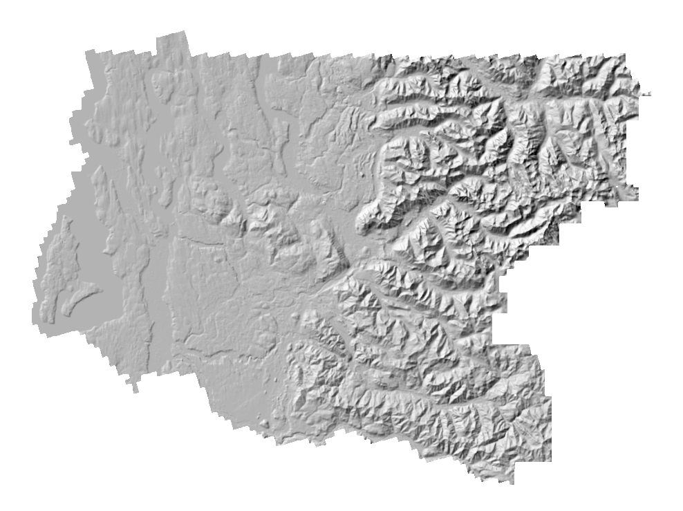
King County DSM Process Step 7: The composite lattice is input to the ArcInfo HILLSHADE command with AZIMUTH = 315, ALTITUDE = 45 and ALL arguments. The output grid is converted to a TIFF image with world file with the GRIDIMAGE command with NONE for colormap and NO on compression to create a default grey-scale hillshade for general use. The composite ArcInfo lattice and Hillshade TIF are inspected for completeness and general overall quality and copied to Data Warehouse. |
| 1/1/2003 |
King County DSM Process Step 2: Digital Surface Model (DSM) .gen files were built for input to the TIN creation function. The .gen files included all points of the subject tile with no buffer of any adjacent tiles. The composite ASCII .gen file was AWKed to create an output file of form: 1,easting, northing, elevation. The constant value of 1 is used to indicate that all points should be treated as Masspoints during the tinning process. The retiled ASCII point files were built into TINs using ArcInfo CREATETIN command with no (0.0) proximity tolerance. |
| 1/1/2003 |
King County DSM Process Step 6: The composite lattice created by merging the individual 7700 tiles extends beyond the extent of the township-range tile. The composite lattice is clipped to the bounds of the township-range tile using the GRID GRIDCLIP function. The resulting clipped lattice is defined with projection information using the PROJECTDEFINE command. |
| 1/1/2003 |
King County DSM Process Step 1: After receipt from 3di Technologies, the data media was cataloged, and the media contents were logged. The ASCII files were retiled into the King County idxp7500 tiling scheme. This resulted in creation of larger files where several 1 x 1 km 3di tiles were appended and clipped to form one 7500 ft x 7500 King County tile. The ASCII records were also appended with a integer identifier resulting in a final record format of identifier, easting, northing, and elevation value. The Puget Sound LiDAR Consortium data included an All-return file that stores points from all LiDAR returns plus operational and timestamp parameters. In the ASCII record was also the RetNo item which was used to extract the first-return records only. |
| 1/1/2003 |
King County DSM Process Step 5: A NULL editmask delineating the open water of the Puget Sound and all areas beyond the project area buffer elsewhere was applied to mask out all remaining 'out-of-bounds' elevation values. This is done mainly to help 'clean-up' the water areas but also cleaned up along the edge of the project area. The boundary used along the shoreline was designed to be conservative to avoid clipping any valid nearshore elevation values. The underlying TINs and ASCII point files can be used to recover, if necessary, any points removed by this edit. |
| 1/1/2002 |
Vendor DSM Production Step 4: First-return point data was transferred to media for delivery to Client in a comma/space delimited ASCII file of format easting,northing,intensity-value. |
| 1/1/2002 |
Vendor DSM Production Step 2: Data by flight line was combined in a merge process that eliminates redundant points. Data was also clipped into more manageable one km x one km bounds. Noise or anomalous returns were filtered from all data during this processing step. The data was quality checked using commercial software, Spectra Precision TerraModel and TerraVista. |
| 1/1/2002 |
Vendor DSM Production Step 3: All elevation data was processed on a point by point basis for ellipsoid to orthometric height conversion using the National Geodetic Survey (NGS) Geoid Model, GEOID99. Datum and coordinate system conversion from WGS84 to the Washington State Plane coordinate system was performed using U.S. Army Corps of Engineers CorpsCon software algorithms. |
| 1/1/2002 |
Vendor DSM Production Step 1: LiDAR data processing was used to produce the x,y,z elevation points using vendor proprietary lidar data processing software. Within this integrated process an atmospheric correction was made, which is especially important in regions of relatively low elevation. |